Spectral features for distinguishing explosions and earthquakes
Frequency composition of seismic events recordings is variable in time. For this reason spectra themself are not very informative for discrimination. Spectral diagrams (sonograms) which illustrate spectrum changes in time are much more informative.
 |
 |
 |
 |
 |
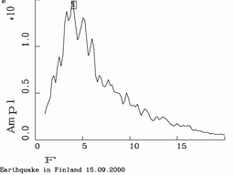 |
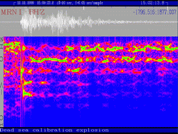
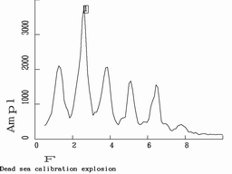
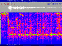
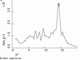
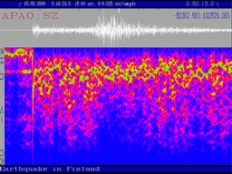
Examples of spectra (right colomn) and sonograms (left) of seismic events. Top plot is calibration explosion in Dead Sea made by Israel Geological Survey (typical recording of underground explosion). Centre plot is recording of Kovdor explosion by Apatity array. Bottom: Northern Finland earthquake.
The figure shows typical spectra and sonograms. (Frequencies in the sonograms increase from top to bottom).
It is noticed that recordings of some explosions have specific bands or belts on sonograms (like Dead See calibration explosion recording). It means that for such explosions special composition is changing in time slowly than for earthquakes (or different explosions).
Although spectra shown in the figure are very different the existance of 'bands' enables to identify the first and second events as explosions. We tried to work out a quantitative measure of such property of a recording as its variability in time.
Suppose we compute correlations between spectral amplitudes calculated for the same recording but for different positions of time window. Let S(w,t) - is spectral amplitude calculated in time window [t-Dt, t+Dt]. Denote C(t1, t2)=corr(S(w ,t1), S(w,t2)). It is obvious that C(t,t)=1 и C(t1,t2)£1.
Now compute average of the correlation A(t)=<C(t,t+t )> by all t inside events recording. Obvious that A(0)=1 and A(t>0)<1. The plot below shows behavior of the functions A(t) for the events mentioned above.
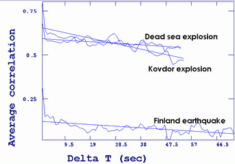
Average correlations A(t) are high for both explosions whereas for the earthquake it falls abruptly and remains at a low level. We guess that for events comparison by A(t) it is not necessary to compare the curves themself but it could be enough to compare linear regressions computed by A in a form A(t)=a+bt. The most informative is a parameter.
The figure below shows some more examples confirming that in many cases explosions could be identified. The following seismic events were processed: recordings of nuclear submarine "Kursk" explosion by Apatity and ARCESS, Apatity recordings of Olenegorsk explosion 31.08.2000 8.58, earthquake near coast of Norway 07.04.2000, 3.40, 67.0 N, 13.9 E, Northern Norway earthquake 21.01.1996, 2.17, 69.9 N, 25.6E.
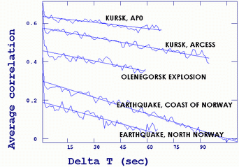
One more test was processing of Kirovsk mine explosions recordings made by ARCESS central vertical sensor. We used 15 large underground explosions, 12 open-pit explosions and 20 compact underground explosions of small yield. For each explosion we computed A(t), and linear regressions in a form A(t)=a+bt. It appeared that 3 groups of explosions differ significantly by a parameter.
|
Kind of explosion |
<a> |
sa |
|
Underground |
0.41 |
0.05 |
|
Open-pit |
0.57 |
0.1 |
|
Compact |
0.28 |
0.1 |
Correlations for compact explosions appeared even less than for large underground although their recordings are very similar. Probably this is due to that compact explosions are much smaller than large underground ones i.e. signal-to-noise ratio is smaller and noise decreases the correlations more significantly.
Currently we made a preliminary program for computing of A(t). The results are still far from perfection. For routine usage of the approch we'll have to work out an optimal computation method and clearify the dependence of the correlations on signal-to-noise ratio. Nevertheless it is obvious that implementation of this parameter will be very useful for seismic events classification.